Signal Analyzer Measurements (1)

1 Initialization (loading Modules and Data)
- 1.1 Helping Tools
- 1.2 Testing
2 Plotting Field dependence of persistend / static field
- 2.1 Crosses
- 2.2 Empty Cross
- 2.3 Measurement Plan #5
3 Field Sweeps
- 3.1 First field Sweeping Experiments
- 3.2 Field Sweeps in Measurement Plan #2
  - 3.2.1 All new measurements together
  - 3.2.2 Δ1 T Sweeps
  - 3.2.3 Compare 2T → 1T
  - 3.2.4 Compare .5 → -.5 T
  - 3.2.5 Group by Sweep Rates (Compare Crosses/Empty)
  - 3.2.6 Low Fields
- 3.3 Measurement Plan #2 / #3
  - 3.3.1 25 mT Sweeps
    - 3.3.1.1 Diff Sweeprates (\(- M_S \rightarrow -25 \rightarrow 25\) mT)
    - 3.3.1.2 SR + Plusses + Empty
    - 3.3.1.3 Temp Effect
  - 3.3.2 Measurement Plan #2
4 Testing
5 Presentation Plots (01 - 2020)

Initialization (loading Modules and Data)

[1]:

# Basic Plotting libraries
import matplotlib.pyplot as plt
import matplotlib
import seaborn as sns
from mpl_toolkits.axes_grid1.inset_locator import inset_axes

# Math / Science Libraries
import pandas as pd
import numpy as np
from scipy import constants, stats

import os, sys, time, re, logging # System Modules
from glob import glob # Readout Files in Directories

# Interactive widgets
import ipywidgets
import IPython
from IPython.display import display

logging.basicConfig(level=logging.WARNING)

%load_ext autoreload

Matplotlib settings for nice plots.

Exports plots without padding margins

[2]:

params = {
    'figure.dpi': 300,
    'figure.figsize': (16,9),
    'figure.subplot.hspace': 0.3,
    'figure.subplot.wspace': 0.3,
    'savefig.transparent': False,
    'savefig.bbox': 'tight',
    'savefig.pad_inches': 0.1,
}
matplotlib.rcParams.update(params)

[3]:

import os
os.getcwd()

[3]:

'/Users/jp/Projects/Code/lab-book/docs/notebooks'

[4]:

os.chdir('../../ana')
os.getcwd()

[4]:

'/Users/jp/Projects/Code/lab-book/ana'

[5]:

import ana
#logging.basicConfig(level=logging.DEBUG)
eva = ana.HandleM(directory='data/SR785/')

WARNING:Handle:Start loading folder: data/SR785/m382_MFN Plusses_T5K_sweep_100 mT to -100 mT_at -1T saturation_Rate 5mTmin_SR785_1.5Hz__aver10_Vin 5V_sens 5mV .dat
WARNING:Handle:Regex doesn't match: data/SR785/MFN_go to zero2.dat
WARNING:Handle:Regex doesn't match: data/SR785/Routine MFN No3.dat
/Users/jp/Projects/Code/lab-book/ana/ana/handle.py:103: DtypeWarning: Columns (0,1,2,3,4,5,6,7,8,9,10,11) have mixed types.Specify dtype option on import or set low_memory=False.
  self.load_folder(file_list, **kwargs)
WARNING:Handle:Regex doesn't match: data/SR785/Test parallel down.dat
WARNING:Handle:Regex doesn't match: data/SR785/Routine MFN.dat
WARNING:Handle:Regex doesn't match: data/SR785/Routine MFN No2.dat
WARNING:Handle:Regex doesn't match: data/SR785/MFN_go to zero.dat
WARNING:Handle:Regex doesn't match: data/SR785/Test2 parallel down.dat
WARNING:Handle:Regex doesn't match: data/SR785/test_n1.dat
WARNING:Handle:Regex doesn't match: data/SR785/test_SR785_length5.dat
WARNING:Handle:Regex doesn't match: data/SR785/test_SR785_length.dat
WARNING:Handle:Regex doesn't match: data/SR785/test_SR785_length4.dat
WARNING:Handle:Regex doesn't match: data/SR785/test_SR785_length6.dat
WARNING:Handle:Regex doesn't match: data/SR785/test.dat
WARNING:Handle:Regex doesn't match: data/SR785/test_SR785_length3.dat
WARNING:Handle:Regex doesn't match: data/SR785/test_SR785_length2.dat
WARNING:Handle:Regex doesn't match: data/SR785/Routine Parallel measurements.dat
WARNING:Handle:Regex doesn't match: data/SR785/f.dat

Helping Tools

Not needed anymore (copied to ana)

[6]:

def get_info(eva):
    info = eva.info
    sa = info[info['type'] == 'SA']
    raw = info[info['type'] == 'RAW']

    vh_idx = []
    mfn_idx = []
    for nr, t in info['technique'].items():
        if 'VH' in t: vh_idx += [nr]
        elif 'MFN' in t: mfn_idx += [nr]
    vh = info.loc[vh_idx]
    mfn = info.loc[mfn_idx]

    groups = dict(vh=vh, mfn=mfn, sa=sa, raw=raw)

    return info, groups

# Set Plotting Style
def set_sns(**style):
    plt.rcParams['savefig.dpi'] = style.get('dpi', 300)
    plt.rcParams['figure.autolayout'] = False
    figsize = style.get('figsize', (8, 6))
    plt.rcParams['figure.figsize'] = figsize
    plt.rcParams['axes.labelsize'] = 18
    plt.rcParams['axes.titlesize'] = 20
    plt.rcParams['font.size'] = 16
    plt.rcParams['lines.linewidth'] = 2.0
    plt.rcParams['lines.markersize'] = 8
    plt.rcParams['legend.fontsize'] = 14
    if style.get('default'):
        %matplotlib inline
        def_size = 'talk'
        def_style = 'darkgrid'
    elif style.get('notebook'):
        %matplotlib notebook
        def_size = 'notebook'
        def_style = 'ticks'


    sns.set(style.get('size', def_size),
            style.get('style', def_style),
            style.get('palette', 'deep'),
            style.get('font', 'sans-serif'),
            style.get('font-scale', 1))

    if style.get('grid'):
        plt.rcParams['axes.grid'] = True
        plt.rcParams['grid.linestyle'] = '--'

    if style.get('latex'):
        plt.rcParams['text.usetex'] = True  # True activates latex output in fonts!
        plt.rcParams[
            'text.latex.preamble'] = ''
    else:
        plt.rcParams['text.usetex'] = False

def set_plot_settings(**kwargs):
    plt.xscale('log')
    plt.yscale('log')

    xmin, xmax = kwargs.get('xlim', (None, None))
    ymin, ymax = kwargs.get('ylim', (None, None))
    if xmin:
        plt.xlim(xmin, xmax)
    if ymin:
        plt.ylim(ymin, ymax)
    plt.legend(loc=kwargs.get('legend_location', 'best'))

set_sns(default=True, grid=True, palette='Set3')

# Set Info
info, groups = get_info(eva)
sa = groups['sa']
raw = groups['raw']
vh = groups['vh']
mfn = groups['mfn']

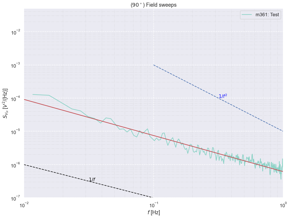
Testing

[7]:

s, i = eva[361].fit()
fig, ax = eva.plot({361: ['Test', {}]})
x = np.logspace(-2, 0, 100)
ax.plot(x, (10**s * np.power(x,i)), 'r-')
#ax.set_xlim()
#ax.set_ylim(1e-7,10)

[7]:

[<matplotlib.lines.Line2D at 0x17d6d9c40>]

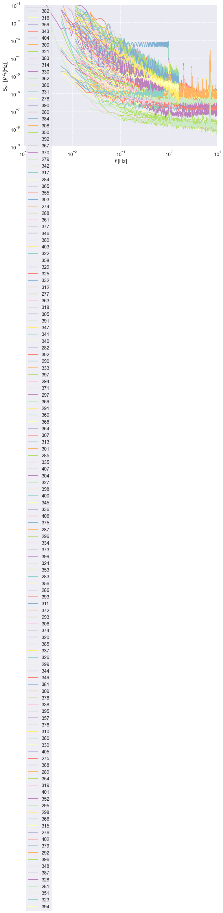
../_images/notebooks_02.1_Signal_Analyzer_12_1.png

[8]:

fig, ax = plt.subplots(figsize=[12,9])
for nr, m in eva.data.items():
    if isinstance(m, ana.SA): # SA Measurement
        m.plot(ax=ax, label=nr)
    elif isinstance(m, ana.RAW): # RAW Measurement
        pass
    #sa[i].plot(label=str(i), ax=ax, dont_set_plot_settings=True)

    # Optionally show Background signal
    #sa[i].plot(plot_y='Vy', label='%s (Vy)' % i[:4], ax=ax)
set_plot_settings(xlim=(1e-3, 1e1), ylim=(1e-9, 1e-1))

../_images/notebooks_02.1_Signal_Analyzer_13_0.png

Field dependence of persistend / static field

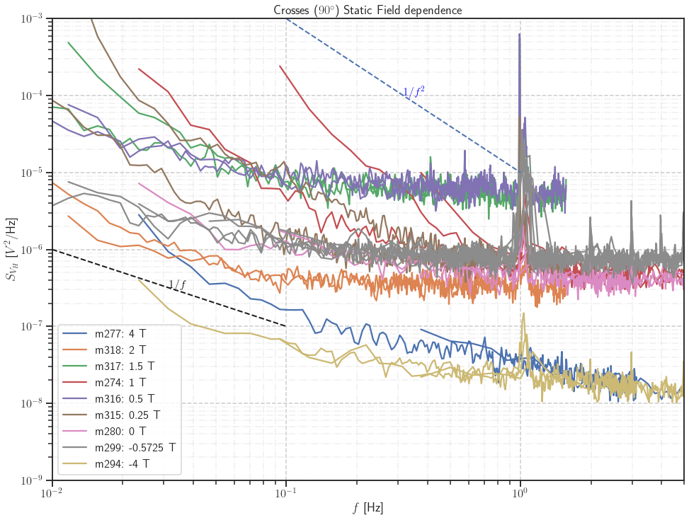
Crosses

[9]:

tmp = {4: 277,
       2: 318,
       1.5: 317,
       1: 274,
       .5: 316,
       .25: 315,
       0: 280,
       -.5725: 299,
       -4: 294, }
lofm = {}
for i, j in tmp.items():
    lofm.update({j: ['%s T' % i, {}]})

set_sns(default=True, grid=True,
        style='ticks',
        #palette='Paired',
        latex=True,)

fig, ax = eva.plot(lofm, plot_settings=dict(title='Crosses ($90^\\circ$) Static Field dependence',
                                            xlim=(1e-2, 5e0),
                                            ylim=(1e-9, 1e-3),
                                           ))

#plt.savefig('img/static_crosses.png', dpi=300)
#plt.savefig('img/static_crosses.pdf', dpi=300)

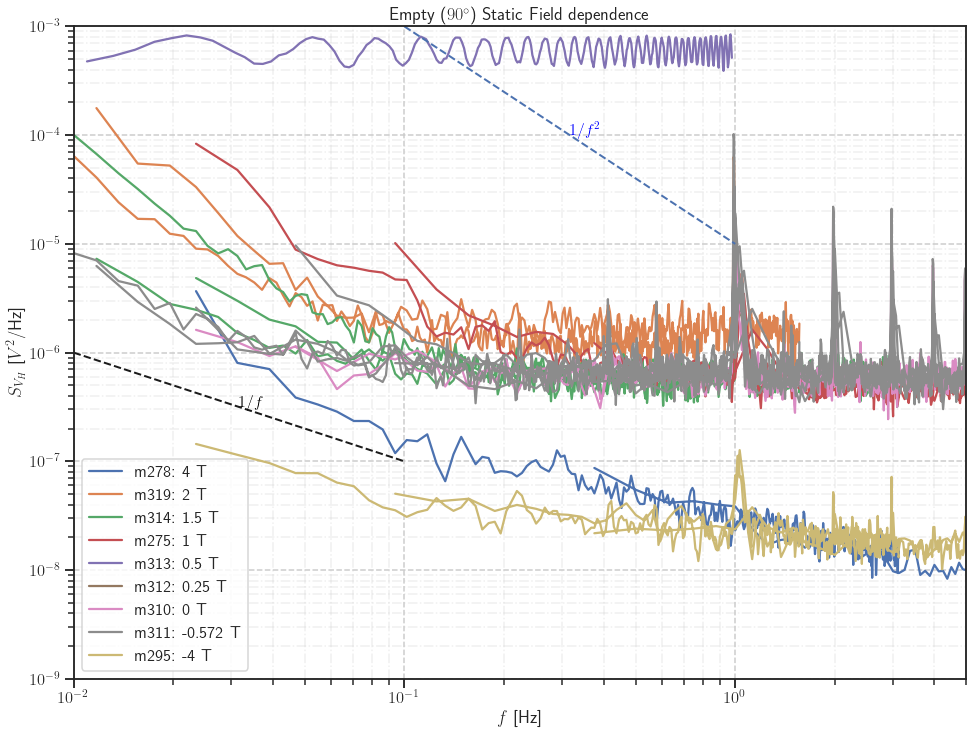
../_images/notebooks_02.1_Signal_Analyzer_16_0.png

Empty Cross

[10]:

tmp = {4: 278,
        2: 319,
      1.5: 314,
        1: 275,
       .5: 313,
      .25: 312,
        0: 310,
    -.572: 311,
        -4: 295,}
lofm = {}

for i, j in tmp.items():
    lofm.update({j: ['%s T' % i, {}]})

set_sns(default=True, grid=True,
        style='ticks',
        #palette='Paired',
        latex=True,)

fig, ax = eva.plot(lofm, plot_settings=dict(title='Empty ($90^\\circ$) Static Field dependence',
                                            xlim=(1e-2, 5e0),
                                            ylim=(1e-9, 1e-3),
                                           ))

#plt.savefig('img/static_empty.png', dpi=300)
#plt.savefig('img/static_empty.pdf', dpi=300)

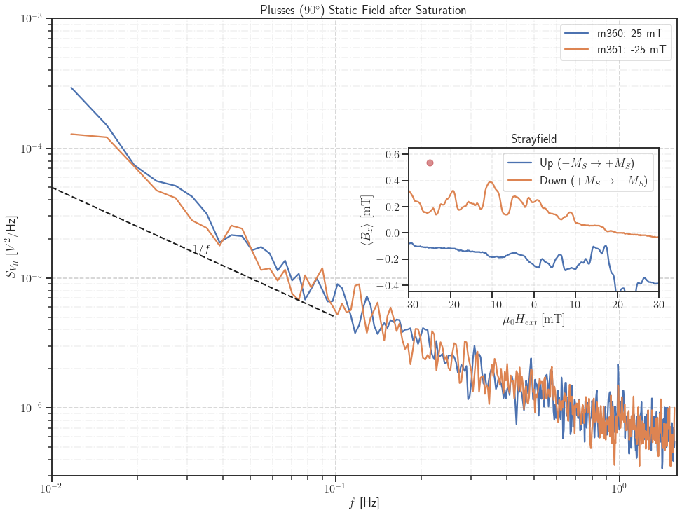
../_images/notebooks_02.1_Signal_Analyzer_18_0.png

Measurement Plan #5

[11]:

sweep_label = '$%s \\rightarrow %s$ T %s ($%s \\frac{mT}{min}$)'
save_figures = False
m = ana.Hloop(57)

[12]:

tmp = {25: 360,
       -25: 361
      }
lofm = {}

for i, j in tmp.items():
    lofm.update({j: ['%s mT' % i, {}]})

set_sns(default=True, grid=True,
        style='ticks',
        #palette='Paired',
        latex=True,)

fig, ax = eva.plot(lofm,
                   fit_range=(2e-2, 1e0),
                   show_fit=False,
                   plot_settings=dict(title='Plusses ($90^\\circ$) Static Field after Saturation',
                                            xlim=(1e-2, 1.6e0),
                                            ylim=(3e-7, 1e-3),
                                           ),
                  f_settings=dict(
                      ymin=5e-5),
                  f2_settings=dict(disable=True))

ax = plt.gca()
with sns.color_palette('deep'):
    inset = inset_axes(ax, width='100%', height='90%',
                       bbox_to_anchor=(.58, .38, .4, .35),
                       bbox_transform=ax.transAxes)
    m.plot_strayfield(inset, 'Strayfield', nolegend=True)
    inset.legend(['Up ($-M_S \\rightarrow +M_S$)', 'Down ($+M_S \\rightarrow -M_S$)'])
    inset.grid(b=True, alpha=.4)
    inset.set_xlim(-30, 30)
    inset.set_ylim(-.45, .65)

    y1, y2 = -1, 2
    a = m.down.Bx8.iloc[(m.down.B + 25).abs().idxmin()]
    b = m.up.Bx8.iloc[(m.up.B - 25).abs().idxmin()]
    inset.plot((-25, -25), (a, a), 'ro', alpha=.4)
    inset.plot([+25, 25], [b,b], 'bo', alpha=.4)

#plt.savefig('img/static_25mT.png')
#plt.savefig('img/static_25mT.pdf')

../_images/notebooks_02.1_Signal_Analyzer_21_0.png

Field Sweeps

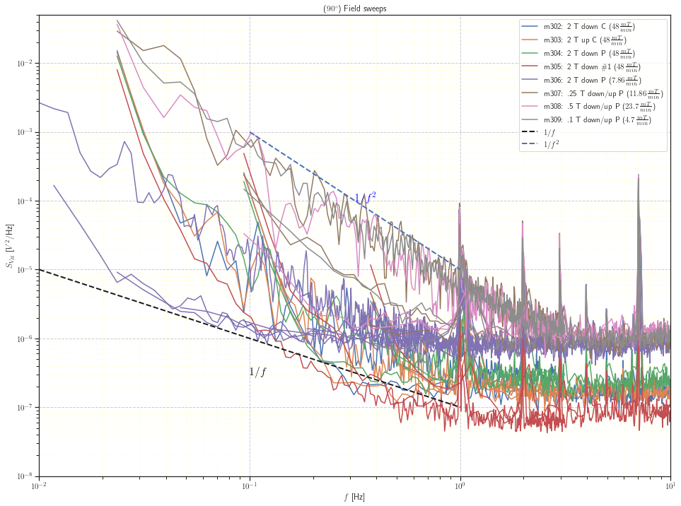
First field Sweeping Experiments

With multiple separate Spectra measured during the sweep.

Measurements 302 - 309

[13]:

lofm = {302: '2 T down C ($48 \\frac{mT}{min}$)',
       303: '2 T up C ($48 \\frac{mT}{min}$)',
       304: '2 T down P ($48 \\frac{mT}{min}$)',
       305: '2 T down \#1 ($48 \\frac{mT}{min}$)',
       306: '2 T down P ($7.86 \\frac{mT}{min}$)',
       307: '.25 T down/up P ($11.86 \\frac{mT}{min}$)',
       308: '.5 T down/up P ($23.7 \\frac{mT}{min}$)',
       309: '.1 T down/up P ($4.7 \\frac{mT}{min}$)',
       }
set_sns(default=True, grid=True, size='notebook', style='ticks', latex=True)

fig, ax = plt.subplots(figsize=(16,12))
for i,j in lofm.items():
    label = 'm%s: %s' % (i, j)
    eva[i].plot(label=label, ax=ax, dont_set_plot_settings=True)


eva[i]._draw_oneoverf(ax, xmin=1e-2, ymin=1e-5, mean_y=3e-7, factor=100)
eva[i]._draw_oneoverf(ax, ymin=1e-3, alpha=2, plot_style='b--', an_color='blue')

eva[i]._set_plot_settings(xlim=(1e-2, 1e1), ylim=(1e-8, 5e-2), title='($90^\circ$) Field sweeps',
                         grid=dict(which='minor', color='#ffff99', linestyle='--', alpha=.3))
#plt.grid(b=True, which='major', color='#cccccc', linestyle='-.')

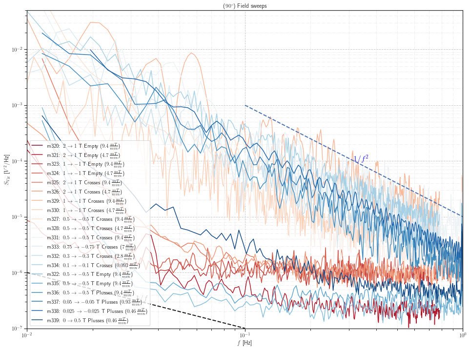
../_images/notebooks_02.1_Signal_Analyzer_24_0.png

Field Sweeps in Measurement Plan #2

One Single Spectrum measured (@1.5 or 0.8 Hz).
25 Averages for single spectrum.

Measurements 320 – 329

All new measurements together

[14]:

#t2 = pd.DataFrame(to_show).T
#t2.columns = ['Fields', 'Struct', 'SR']
#g = t2.groupby('Struct')
#set_sns(default=True, grid=True, size='notebook', style='ticks', latex=True,
#        palette='Dark2')

#for key, group in g:
#    lofm = eva.get_lofm(group, '$%s \\rightarrow %s$ T %s ($%s \\frac{mT}{min}$)')
#    eva.plot(lofm)

[15]:

to_show = {
    320: [(2,1), 'Empty', 9.4],
    321: [(2,1), 'Empty', 4.7],
    323: [(1,-1), 'Empty', 9.4],
    324: [(1,-1), 'Empty', 4.7],
    325: [(2,1), 'Crosses', 9.4],
    326: [(2,1), 'Crosses', 4.7],
    329: [(1,-1), 'Crosses', 9.4],
    330: [(1,-1), 'Crosses', 4.7],
    327: [(.5,-.5), 'Crosses', 9.4],
    328: [(.5,-.5), 'Crosses', 4.7],
    331: [(.5,-.5), 'Crosses', 9.4],
    333: [(.75,-.75), 'Crosses', 7],
    332: [(.3,-.3), 'Crosses', 2.8],
    334: [(.1,-.1), 'Crosses', .093],
    322: [(.5,-.5), 'Empty', 9.4],
    335: [(.5,-.5), 'Empty', 9.4],
    336: [(.5,-.5), 'Plusses', 9.4],
    337: [(.05,-.05), 'Plusses', 0.93],
    338: [(.025,-.025), 'Plusses', 0.46],
    339: [(0,.5), 'Plusses', 0.46],
    #302: [(2,-2), 'Crosses', 48],
    #303: [(-2,2), 'Crosses', 48],
    #305: [(2,-2), 'Empty', 48],
}

lofm = eva.get_lofm_sweeps(to_show, '$%s \\rightarrow %s$ T %s ($%s \\frac{mT}{min}$)')

set_sns(default=True, grid=True, size='notebook', style='ticks', latex=True,
        palette='Dark2')

with sns.color_palette("RdBu", n_colors=20):
    eva.plot(lofm)

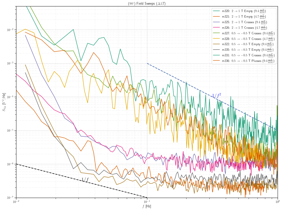
../_images/notebooks_02.1_Signal_Analyzer_28_0.png

Δ1 T Sweeps

[16]:

lofm = {}
to_show = {
    320: [(2,1), 'Empty', 9.4],
    321: [(2,1), 'Empty', 4.7],
    325: [(2,1), 'Crosses', 9.4],
    326: [(2,1), 'Crosses', 4.7],
    327: [(.5,-.5), 'Crosses', 9.4],
    328: [(.5,-.5), 'Crosses', 4.7],
    322: [(.5,-.5), 'Empty', 9.4],
    335: [(.5,-.5), 'Empty', 9.4],
    331: [(.5,-.5), 'Crosses', 9.4],
    336: [(.5,-.5), 'Plusses', 9.4],
}

for nr, content in to_show.items():
    lofm[nr] = [sweep_label % (
                content[0][0],
                content[0][1],
                content[1],
                content[2],
                ),{}]

#lofm = eva.get_lofm_sweeps(to_show, '$%s \\rightarrow %s$ T %s ($%s \\frac{mT}{min}$)')

set_sns(default=True, grid=True, size='notebook', style='ticks', latex=True,
        palette='Dark2')

eva.plot(lofm, plot_settings=dict(title='($90^\\circ$) Field Sweeps ($\\Delta 1 T$)'))
#plt.savefig('img/sweep_delta1T.png', dpi=300)
#plt.savefig('img/sweep_delta1T.pdf', dpi=300)


#eva[i]._set_plot_settings(xlim=(1e-2, 1e0), ylim=(1e-7, 5e-2), title='($90^\circ$) Field sweeps',
#                         grid=dict(which='minor', color='#ffff99', linestyle='--', alpha=.5))
#plt.grid(b=True, which='minor', color='#cccccc', linestyle='-.', alpha=.3)

[16]:

(<Figure size 1152x864 with 1 Axes>,
 <AxesSubplot:title={'center':'($90^\\circ$) Field Sweeps ($\\Delta 1 T$)'}, xlabel='$f$ [Hz]', ylabel='$S_{V_H}$ [${V^2}$/{Hz}]'>)

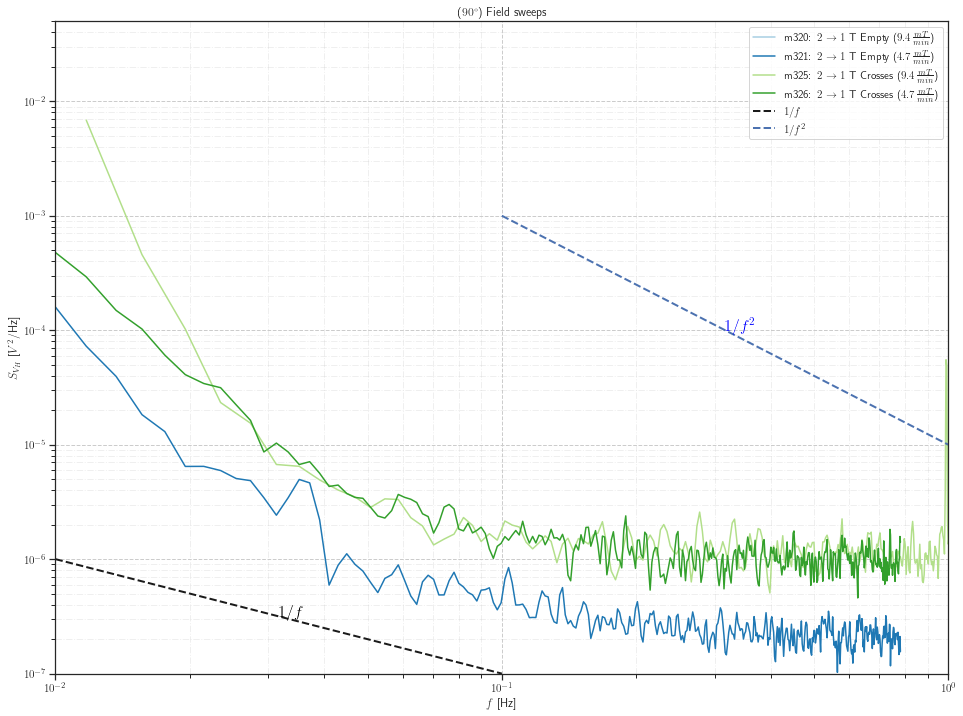
../_images/notebooks_02.1_Signal_Analyzer_30_1.png

Compare 2T → 1T

[17]:

lofm = {}
to_show = {
    320: [(2,1), 'Empty', 9.4],
    321: [(2,1), 'Empty', 4.7],
#    323: [(1,-1), 'Empty', 9.4],
#    324: [(1,-1), 'Empty', 4.7],
    325: [(2,1), 'Crosses', 9.4],
    326: [(2,1), 'Crosses', 4.7],
#    327: [(.5,-.5), 'Crosses', 9.4],
#    328: [(.5,-.5), 'Crosses', 4.7],
#    329: [(1,-1), 'Crosses', 9.4],
#    322: [(.5,-.5), 'Empty', 9.4],
}

for nr, content in to_show.items():
    lofm[nr] = '$%s \\rightarrow %s$ T %s ($%s \\frac{mT}{min}$)' % (
                content[0][0],
                content[0][1],
                content[1],
                content[2],
                )

set_sns(default=True, grid=True, size='notebook', style='ticks', latex=True, palette='Paired')
#sns.set(pal)
fig, ax = plt.subplots(figsize=(16,12))
for i,j in lofm.items():
    label = 'm%s: %s' % (i, j)
    eva[i].plot(label=label, ax=ax, dont_set_plot_settings=True)


eva[i]._draw_oneoverf(ax, xmin=1e-2, ymin=1e-6)
eva[i]._draw_oneoverf(ax, ymin=1e-3, alpha=2, plot_style='b--', an_color='blue')

eva[i]._set_plot_settings(xlim=(1e-2, 1e0), ylim=(1e-7, 5e-2), title='($90^\circ$) Field sweeps',
                         grid=dict(which='minor', color='#ffff99', linestyle='--', alpha=.5))
plt.grid(b=True, which='minor', color='#cccccc', linestyle='-.', alpha=.3)

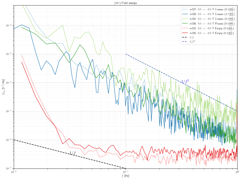
../_images/notebooks_02.1_Signal_Analyzer_32_0.png

Compare .5 → -.5 T

[18]:

lofm = {}
to_show = {
    327: [(.5,-.5), 'Crosses', 9.4],
    328: [(.5,-.5), 'Crosses', 4.7],
    331: [(.5,-.5), 'Crosses', 9.4],
    336: [(.5,-.5), 'Plusses', 9.4],
    322: [(.5,-.5), 'Empty', 9.4],
    335: [(.5,-.5), 'Empty', 9.4],
}

for nr, content in to_show.items():
    lofm[nr] = '$%s \\rightarrow %s$ T %s ($%s \\frac{mT}{min}$)' % (
                content[0][0],
                content[0][1],
                content[1],
                content[2],
                )

set_sns(default=True, grid=True, size='notebook', style='ticks', latex=True,
        palette='Paired')
#sns.set(pal)
fig, ax = plt.subplots(figsize=(16,12))
for i,j in lofm.items():
    label = 'm%s: %s' % (i, j)
    eva[i].plot(label=label, ax=ax, dont_set_plot_settings=True)


eva[i]._draw_oneoverf(ax, xmin=1e-2, ymin=1e-6)
eva[i]._draw_oneoverf(ax, ymin=1e-3, alpha=2, plot_style='b--', an_color='blue')

eva[i]._set_plot_settings(xlim=(1e-2, 1e0), ylim=(1e-7, 5e-2), title='($90^\circ$) Field sweeps',
                         grid=dict(which='minor', color='#ffff99', linestyle='--', alpha=.5))
plt.grid(b=True, which='minor', color='#cccccc', linestyle='-.', alpha=.3)

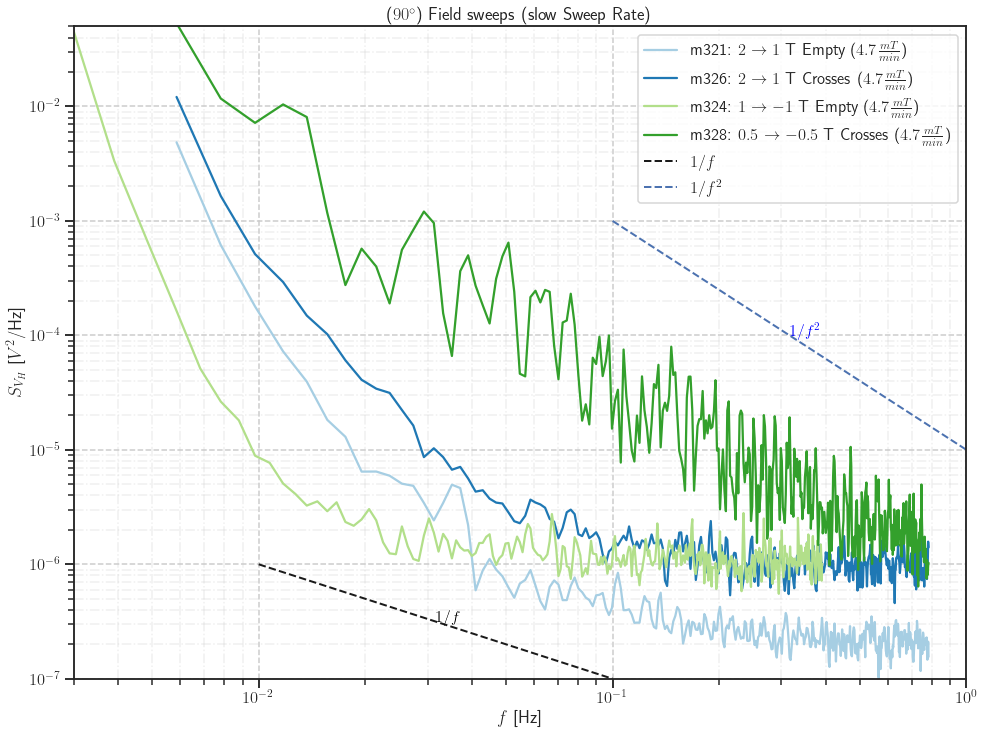
../_images/notebooks_02.1_Signal_Analyzer_34_0.png

Group by Sweep Rates (Compare Crosses/Empty)

Slow Sweeprate

[19]:

lofm = {}
to_show = {
    320: [(2,1), 'Empty', 9.4],
    321: [(2,1), 'Empty', 4.7],
    325: [(2,1), 'Crosses', 9.4],
    326: [(2,1), 'Crosses', 4.7],
    323: [(1,-1), 'Empty', 9.4],
    324: [(1,-1), 'Empty', 4.7],
    329: [(1,-1), 'Crosses', 9.4],
    322: [(.5,-.5), 'Empty', 9.4],
    327: [(.5,-.5), 'Crosses', 9.4],
    328: [(.5,-.5), 'Crosses', 4.7],
    336: [(.5,-.5), 'Plusses', 9.4],
}

for nr, content in to_show.items():
    if content[2] == 9.4:
        continue
    lofm[nr] = '$%s \\rightarrow %s$ T %s ($%s \\frac{mT}{min}$)' % (
                content[0][0],
                content[0][1],
                content[1],
                content[2],
                )

set_sns(default=True, grid=True, size='talk', style='ticks', latex=True, palette='Paired')
#sns.set(pal)
fig, ax = plt.subplots(figsize=(16,12))
for i,j in lofm.items():
    label = 'm%s: %s' % (i, j)
    if i == 336:
        eva[i].plot(label=label, ax=ax, color='yellow', dont_set_plot_settings=True)

    eva[i].plot(label=label, ax=ax, dont_set_plot_settings=True)


eva[i]._draw_oneoverf(ax, xmin=1e-2, ymin=1e-6)
eva[i]._draw_oneoverf(ax, ymin=1e-3, alpha=2, plot_style='b--', an_color='blue')

eva[i]._set_plot_settings(xlim=(3e-3, 1e0), ylim=(1e-7, 5e-2),
                          title='($90^\circ$) Field sweeps (slow Sweep Rate)',
                          grid=dict(which='minor', color='#ffff99', linestyle='--', alpha=.5))
plt.grid(b=True, which='minor', color='#cccccc', linestyle='-.', alpha=.3)

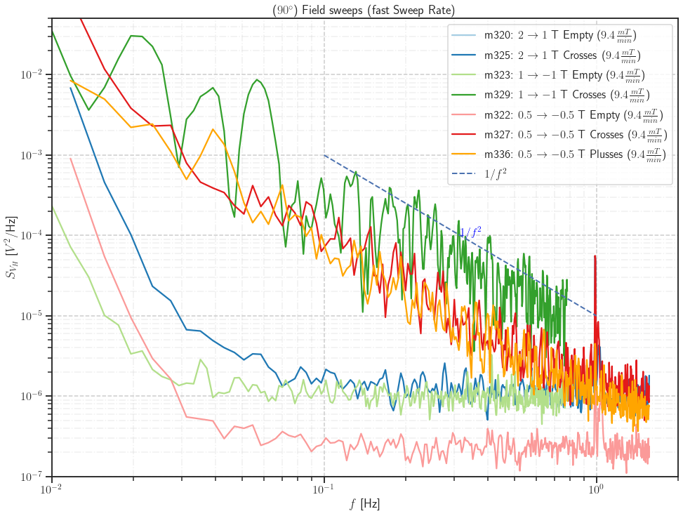
../_images/notebooks_02.1_Signal_Analyzer_37_0.png

Fast Sweeprate

[20]:

lofm = {}
for nr, content in to_show.items():
    if content[2] == 4.7:
        continue
    lofm[nr] = '$%s \\rightarrow %s$ T %s ($%s \\frac{mT}{min}$)' % (
                content[0][0],
                content[0][1],
                content[1],
                content[2],
                )

set_sns(default=True, grid=True, size='talk', style='ticks', latex=True, palette='Paired')
#sns.set(pal)
fig, ax = plt.subplots(figsize=(16,12))
for i,j in lofm.items():
    label = 'm%s: %s' % (i, j)
    if i == 336:
        eva[i].plot(label=label, ax=ax, color='orange', dont_set_plot_settings=True)
    else:
        eva[i].plot(label=label, ax=ax, dont_set_plot_settings=True)


#eva[i]._draw_oneoverf(ax, xmin=1e-2, ymin=1e-6)
eva[i]._draw_oneoverf(ax, ymin=1e-3, alpha=2, plot_style='b--', an_color='blue')

eva[i]._set_plot_settings(xlim=(1e-2, 2e0), ylim=(1e-7, 5e-2), title='($90^\circ$) Field sweeps (fast Sweep Rate)',
                         grid=dict(which='minor', color='#ffff99', linestyle='--', alpha=.5))
plt.grid(b=True, which='minor', color='#cccccc', linestyle='-.', alpha=.3)

plt.savefig('FastSR.pdf', bbox_inches='tight')

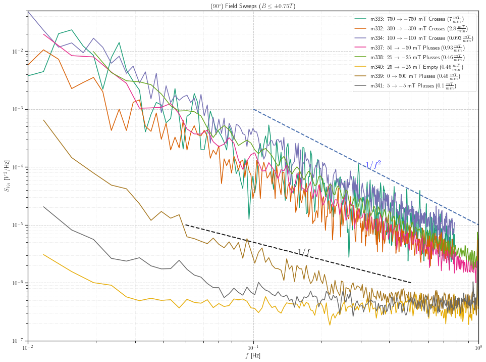
../_images/notebooks_02.1_Signal_Analyzer_39_0.png

Low Fields

[21]:

lofm = {}
to_show = {
    333: [(.75,-.75), 'Crosses', 7],
    332: [(.3,-.3), 'Crosses', 2.8],
    334: [(.1,-.1), 'Crosses', .093],
    337: [(.05,-.05), 'Plusses', 0.93],
    338: [(.025,-.025), 'Plusses', 0.46],
    340: [(.025,-.025), 'Empty', 0.46],
    339: [(0,.5), 'Plusses', 0.46],
    341: [(.005, -.005), 'Plusses', 0.1]
}

for nr, content in to_show.items():
    if content[2] == 9.4:
        continue
    lofm[nr] = ['$%d \\rightarrow %d$ mT %s ($%s \\frac{mT}{min}$)' % (
                content[0][0]*1e3,
                content[0][1]*1e3,
                content[1],
                content[2],
                ),{}]

set_sns(default=True, grid=True, size='notebook', style='ticks', latex=True,
        palette='Dark2')

eva.plot(lofm, plot_settings=dict(title='($90^\\circ$) Field Sweeps ($B \\leq \\pm 0.75 T$)'),
        f_settings=dict(xmin=5e-2, ymin=1e-5))
#plt.savefig('img/sweep_lowfield.png', dpi=300)
#plt.savefig('img/sweep_lowfield.pdf', dpi=300)

[21]:

(<Figure size 1152x864 with 1 Axes>,
 <AxesSubplot:title={'center':'($90^\\circ$) Field Sweeps ($B \\leq \\pm 0.75 T$)'}, xlabel='$f$ [Hz]', ylabel='$S_{V_H}$ [${V^2}$/{Hz}]'>)

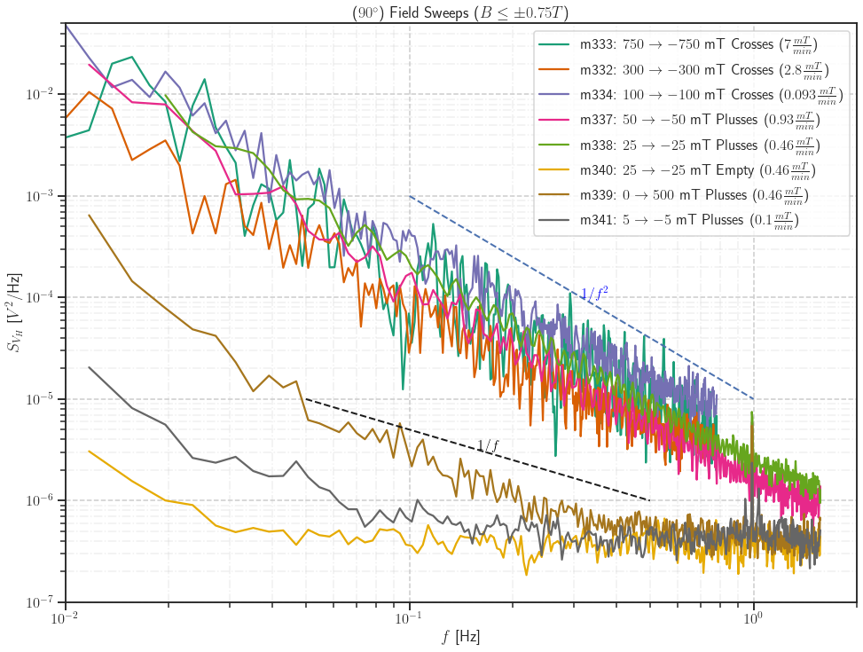
../_images/notebooks_02.1_Signal_Analyzer_41_1.png

[23]:

set_sns(default=True, grid=True, size='talk', style='ticks', latex=True,
        palette='Dark2')

eva.plot(lofm,
         plot_settings=dict(
             title='($90^\\circ$) Field Sweeps ($B \\leq \\pm 0.75 T$)',
             xlim=(1e-2, 2e0)),
         f_settings=dict(
             xmin=5e-2,
             ymin=1e-5))
#plt.savefig('img/sweep_lowfield2.png', dpi=300)
#plt.savefig('img/sweep_lowfield2.pdf', dpi=300)

[23]:

(<Figure size 1152x864 with 1 Axes>,
 <AxesSubplot:title={'center':'($90^\\circ$) Field Sweeps ($B \\leq \\pm 0.75 T$)'}, xlabel='$f$ [Hz]', ylabel='$S_{V_H}$ [${V^2}$/{Hz}]'>)

../_images/notebooks_02.1_Signal_Analyzer_42_1.png

Measurement Plan #2 / #3

25 mT Sweeps

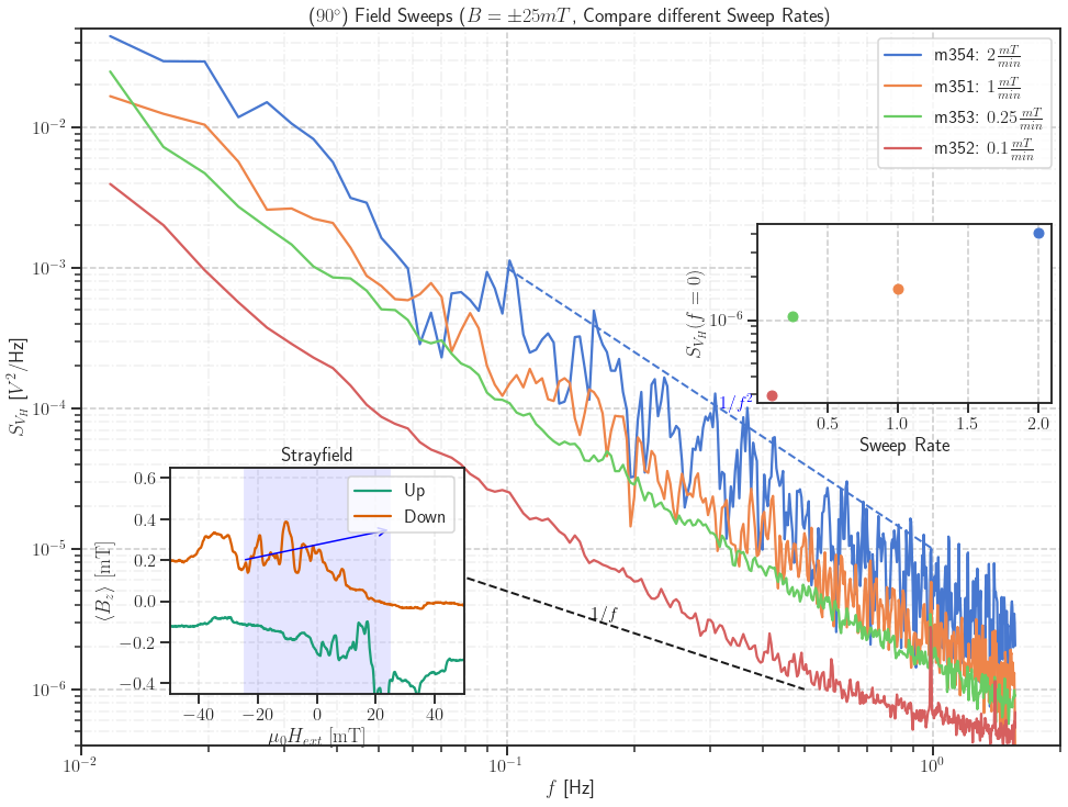
Diff Sweeprates (\(- M_S \rightarrow -25 \rightarrow 25\) mT)

[24]:

set_sns(default=True, grid=True, size='talk', style='ticks', latex=True,
        palette='muted')
#sns.color_palette('muted', 4)

lofm = {}
to_show = {
    354: [("-M_s \\rightarrow -25",25), 'Plusses', 2],
    351: [("-M_s \\rightarrow -25",25), 'Plusses', 1],
    353: [("-M_s \\rightarrow -25",25), 'Plusses', .25],
    352: [("-M_s \\rightarrow -25",25), 'Plusses', .1],
}

for nr, content in to_show.items():
    lofm[nr] = ["$%s \\frac{mT}{min}$" % (
                content[2],
                ),{}]


eva.plot(lofm,
       #fit_range=(2e-2, 5e-1),
       #show_fit=False,
         plot_settings=dict(
             title='($90^\\circ$) Field Sweeps ($B = \\pm 25 mT$, Compare different Sweep Rates)',
             xlim=(1e-2, 2e0),
             ylim=(4e-7, 5e-2)),
         f_settings=dict(
             xmin=5e-2,
             ymin=1e-5))

ax = plt.gca()
with sns.color_palette('Dark2'):
    inset = inset_axes(ax, width='100%', height='90%',
                       bbox_to_anchor=(.1, .05, .3, .35),
                       bbox_transform=ax.transAxes)
    m.plot_strayfield(inset, 'Strayfield', nolegend=True)
    inset.legend(['Up',# ($-M_S \\rightarrow +M_S$)',
                  'Down'])# ($+M_S \\rightarrow -M_S$)'])
    inset.grid(b=True, alpha=.4)
    inset.set_xlim(-50, 50)
    inset.set_ylim(-.45, .65)

    y1, y2 = -1, 2
    inset.fill([-25, -25, 25, 25], [y1, y2, y2, y1], 'blue', alpha=.1)
    #inset.plot([8.3, 8.3], [y1, y2], 'b-.', alpha=.4)
    inset.annotate("", xy=(25, .35), xytext=(-25, .2),
                 arrowprops=dict(arrowstyle="->", color='blue'))
with sns.color_palette('muted'):
    inset2 = inset_axes(ax, width='100%', height='100%',
                       bbox_to_anchor=(.7, .49, .3, .25),
                       bbox_transform=ax.transAxes)

    for nr, content in to_show.items():
        intercept, slope = eva[nr].fit(fit_range=(2e-2, 5e-1))
        sweep_rate = content[2]

        inset2.plot(sweep_rate, 10**intercept, 'o')

    inset2.set_xlabel('Sweep Rate')
    inset2.set_ylabel('$S_{V_H} (f=0)$')
    inset2.set_yscale('log')

# Only save if necessary
plt.savefig('sweeprate-effect.pdf', bbox_inches='tight', dpi=300)
if save_figures:
    plt.savefig('img/sweep_25mT_SR.png', dpi=300)
    plt.savefig('img/sweep_25mT_SR.pdf', dpi=300)

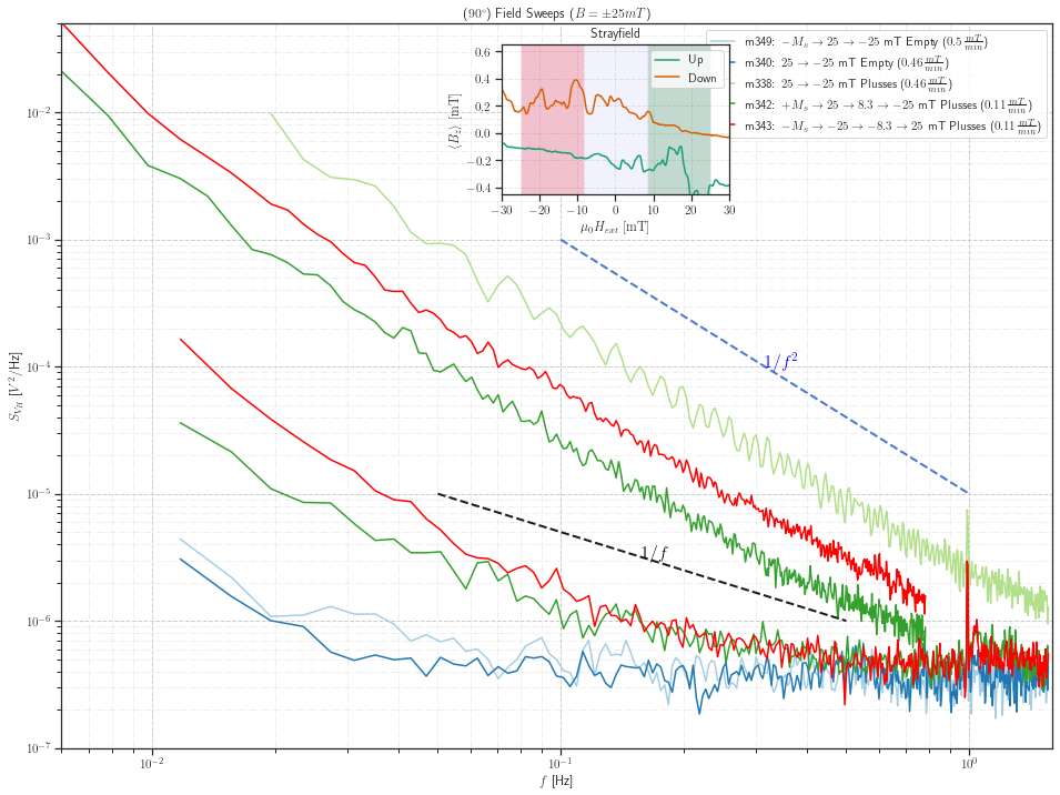
../_images/notebooks_02.1_Signal_Analyzer_46_0.png

SR + Plusses + Empty

[25]:

set_sns(default=True, grid=True, size='notebook', style='ticks', latex=True,
        palette='Paired')

lofm = {}
to_show = {
    349: [("-M_s \\rightarrow 25",-25), 'Empty', 0.5, {}],
    340: [(25,-25), 'Empty', 0.46, {}],
    338: [(25,-25), 'Plusses', 0.46, {}],
    342: [("+M_s \\rightarrow 25 \\rightarrow 8.3",-25), 'Plusses', +0.11, {}],
    343: [("-M_s \\rightarrow -25 \\rightarrow -8.3",25), 'Plusses', 0.11, {'color': 'red'}],
}

for nr, content in to_show.items():
    if content[2] == 9.4:
        continue
    lofm[nr] = ['$%s \\rightarrow %s$ mT %s ($%s \\frac{mT}{min}$)' % (
                content[0][0],
                content[0][1],
                content[1],
                content[2],
                ),content[3]]

eva.plot(lofm,
         plot_settings=dict(
             title='($90^\\circ$) Field Sweeps ($B = \\pm 25 mT$)',
             xlim=(6e-3, 1.6e0),
             #ylim=()
         ),
         f_settings=dict(
             xmin=5e-2,
             ymin=1e-5))

ax = plt.gca()
with sns.color_palette('Dark2'):
    inset = inset_axes(ax, width='100%', height='90%',
                       bbox_to_anchor=(.45, .75, .23, .23),
                       bbox_transform=ax.transAxes)
    m.plot_strayfield(inset, 'Strayfield', nolegend=True)
    inset.legend(['Up', 'Down'])
    inset.grid(b=True, alpha=.4)
    inset.set_xlim(-30, 30)
    inset.set_ylim(-.45, .65)

    y1, y2 = -1, 2
    inset.fill([-25, -25, -8.3, -8.3], [y1, y2, y2, y1], 'red', alpha=.2)
    inset.fill([25, 25, 8.3, 8.3], [y1, y2, y2, y1], 'green', alpha=.2)
    inset.fill([25, 25, -25, -25], [y1, y2, y2, y1], 'blue', alpha=.05)
    #inset.plot([8.3, 8.3], [y1, y2], 'b-.', alpha=.8)

# Only save if necessary
if save_figures:
    plt.savefig('img/sweep_25mT.png', dpi=300)
    plt.savefig('img/sweep_25mT.pdf', dpi=300)

../_images/notebooks_02.1_Signal_Analyzer_48_0.png

Temp Effect

[26]:

set_sns(default=True, grid=True, size='notebook', style='ticks', latex=True,
        palette='muted')

lofm = {}
to_show = {
    355: [("-M_s \\rightarrow -25",25), 'Plusses', 0.5, 25],
    356: [("-M_s \\rightarrow -25",25), 'Plusses', 0.5, 20],
    #357: [("-M_s \\rightarrow -25",25), 'Plusses', 0.5, 15],
    358: [("-M_s \\rightarrow -25",25), 'Plusses', 0.5, 10],
    359: [("-M_s \\rightarrow -25",25), 'Plusses', 0.5, 5],
}

for nr, content in to_show.items():
    lofm[nr] = ['$%s\\, K$' % (
                content[3],
                ),{}]

t = '($90^\\circ$) Field Sweeps ($B = \\pm 25 mT$) ' + \
    '$%s \\rightarrow %s$ mT %s ($%s \\frac{mT}{min}$)' % (
                content[0][0],
                content[0][1],
                content[1],
                content[2])
eva.plot(lofm,
         plot_settings=dict(
             title=t,
             xlim=(1e-2, 1.6e0),
             ylim=(6e-7, 5e-2)
         ),
         f_settings=dict(
             xmin=5e-2,
             ymin=1e-5, disable=True))

# Only save if necessary
if save_figures:
    plt.savefig('img/sweep_25mT_T.png', dpi=300)
    plt.savefig('img/sweep_25mT_T.pdf', dpi=300)

../_images/notebooks_02.1_Signal_Analyzer_50_0.png

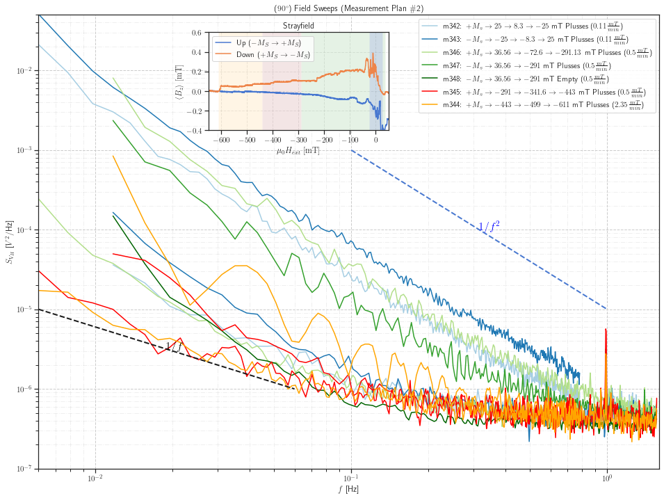
Measurement Plan #2

[27]:

plt.style.use('ggplot')
set_sns(default=True, grid=True, size='notebook', style='ticks', latex=True,
        palette='Paired')
lofm = {}
to_show = {
    342: [("+M_s \\rightarrow 25 \\rightarrow 8.3",-25), 'Plusses', +0.11, {}],
    343: [("-M_s \\rightarrow -25 \\rightarrow -8.3",25), 'Plusses', 0.11, {}],
    346: [("+M_s \\rightarrow 36.56 \\rightarrow -72.6",-291.13), 'Plusses', 0.5,{}],
    347: [("-M_s \\rightarrow 36.56",-291), 'Plusses', 0.5,{}],
    348: [("-M_s \\rightarrow 36.56",-291), 'Empty', 0.5, {'color': 'darkgreen'}],
    345: [("+M_s \\rightarrow -291 \\rightarrow -341.6",-443), 'Plusses', 0.5, {'color': 'red'}],
    344: [("+M_s \\rightarrow -443 \\rightarrow -499",-611), 'Plusses', +2.35, {'color': 'orange'}],
}

for nr, content in to_show.items():
    if content[2] == 9.4:
        continue
    options = content[3]
    lofm[nr] = ['$%s \\rightarrow %s$ mT %s ($%s \\frac{mT}{min}$)' % (
                content[0][0],
                content[0][1],
                content[1],
                content[2],
                ),options]

eva.plot(lofm,
         plot_settings=dict(
             title='($90^\\circ$) Field Sweeps (Measurement Plan \#2)',
             xlim=(6e-3, 1.6e0),
             #ylim=()
         ),
         f_settings=dict(
             xmin=6e-3,
             ymin=1e-5))

ax = plt.gca()
with sns.color_palette('muted'):
    inset = inset_axes(ax, width='100%', height='90%',
                       bbox_to_anchor=(.28, .73, .29, .24),
                       bbox_transform=ax.transAxes)
    m.plot_strayfield(inset, 'Strayfield', nolegend=True)
    inset.legend(['Up ($-M_S \\rightarrow +M_S$)', 'Down ($+M_S \\rightarrow -M_S$)'])
    inset.grid(b=True, alpha=.4)
    inset.set_xlim(-650, 50)
    inset.set_ylim(-.4, .6)

    y1, y2 = -1, 2
    inset.fill([-25, -25, 25, 25], [y1, y2, y2, y1], 'blue', alpha=.1)
    inset.fill([-291.13, -291.13, 36.56, 36.56], [y1, y2, y2, y1], 'green', alpha=.1)
    inset.fill([-611, -611, -443, -443], [y1, y2, y2, y1], 'orange', alpha=.1)
    inset.fill([-291, -291, -443, -443], [y1, y2, y2, y1], 'darkred', alpha=.1)


# Only save if necessary
#plt.savefig('sweep_measplan2.png', dpi=300)
#if save_figures:
#    plt.savefig('img/sweep_measplan2.png', dpi=300)
#    plt.savefig('img/sweep_measplan2.pdf', dpi=300)

../_images/notebooks_02.1_Signal_Analyzer_52_0.png

[ ]:

Signal Analyzer Measurements (1)

Table of Contents

Initialization (loading Modules and Data)

Helping Tools

Testing

Field dependence of persistend / static field

Crosses

Empty Cross

Measurement Plan #5

Field Sweeps

First field Sweeping Experiments

Field Sweeps in Measurement Plan #2

All new measurements together

Δ1 T Sweeps

Compare 2T → 1T

Compare .5 → -.5 T

Group by Sweep Rates (Compare Crosses/Empty)

Slow Sweeprate

Fast Sweeprate

Low Fields

Measurement Plan #2 / #3

Diff Sweeprates (\(- M_S \rightarrow -25 \rightarrow 25\) mT)

SR + Plusses + Empty

Temp Effect

Measurement Plan #2